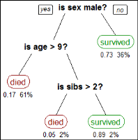
A decision tree predicts the class of an object based on the object’s attributes. For example, you can use a decision tree to predict whether a passenger on the Titanic survived, based on the passenger’s gender, age, and number of siblings, as shown in Figure 6‑11. The numbers under each leaf show the probability of survival for a passenger with the specified attributes and the percentage of passengers represented by the leaf. Figure 6‑11 tells us:
A female passenger had a 0.73 chance of surviving.
A male passenger over the age of 9 had only a 0.17 chance of surviving.
For male passengers age 9 or younger, the probability of survival depends on the number of siblings the passenger had. If the passenger had more than two siblings, he had only a 0.05 chance of surviving. If the passenger had two siblings or fewer, he had a 0.89 chance of surviving.
Figure 6‑11 Decision tree showing survival probabilities for passengers on the Titanic
Figure 6‑14 shows a decision tree that predicts whether a worker is low income, medium income, or high income, based on the worker’s occupation and gender.
Training and testing a predictive model
A decision tree must be trained on sample data. The decision tree learns with each successive application of the predictive model. Some patterns found by data mining algorithms, however, are invalid. Data mining algorithms often find patterns in the training set that are not present in the general data set. This is called overfitting.
To solve this problem, test the predictive model on a set of data different from the training set. The learned patterns are applied to the test set and the resulting output is compared to the desired output. For example, a data mining algorithm that distinguishes spam from legitimate e-mails is trained on a set of sample e-mails. Once trained, the learned patterns are applied to a test set of emails. The accuracy of the predictive model is measured from how many e-mails it classifies correctly.
Understanding the confusion matrix
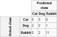
A confusion matrix tabulates the results of a predictive algorithm. Each row of the matrix represents an actual class. Each column represents a predicted class. For example, consider a classification system that has been trained to distinguish between cats, dogs, and rabbits.
Figure 6‑12 shows how frequently the predictive algorithm correctly classifies each type of animal. The sample contains 27 animals: 8 cats, 6 dogs, and 13 rabbits. Of the 8 cats, the algorithm predicted that three are dogs, and of the six dogs, it predicted that two are cats and one is a rabbit. The confusion matrix shows that the algorithm is not very successful distinguishing between cats and dogs. It is, however, successful distinguishing between rabbits and other types of animals, misclassifying only two of 13 rabbits. Correct predictions are tallied in the table’s diagonal. Non-zero values outside the diagonal indicate incorrect predictions.
Figure 6‑12 Confusion matrix showing the actual class and predicted class for animals
Understanding sensitivity and specificity
Sensitivity, also called the true positive rate, measures the proportion of actual positives that are correctly identified as such, for example the percentage of sick people who are correctly identified as having a condition. Specificity, also called the true negative rate, measures the proportion of negatives that are correctly identified as such, for example the percentage of healthy people who are correctly identified as not having a condition.
A perfect predictor is 100% sensitive, in other words predicting that all people in the sick group are sick, and 100% specific, in other words not predicting that anyone in the healthy group is sick. For any test, however, there is a trade-off between the measures. For example, in an airport security setting where one is testing for potential threats to safety, scanners may be set to trigger on low-risk items such as belt buckles and keys, low specificity, to reduce the risk of missing objects that pose a threat to passengers and crew, high sensitivity.
How to create a decision tree
1 In Analytics—Advanced, choose Decision tree.
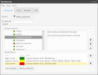
2 Drag the appropriate table from My Data and drop it in Domain in Decision tree, shown in Figure 6‑13.
Figure 6‑13 Specifying the parameters for a decision tree
3 In the left pane of Domain columns, expand the database and the appropriate tables.
4 Drag the appropriate columns from the left pane and drop them in the right pane. The columns specify the attributes used to assign classifications in the decision tree.
5 Create the classifications:
1 Choose New classifier.
2 In Alias, type the name of the classifier.
3 Choose the color picker button and select a color. The name and the color visually identify the classification in the decision tree. For example, you can define a High income classification identified by the color green.
4 Drag a segment from Discrete values and drop it in Drag a segment. The segment specifies the condition for the classification. For example, you can define a High income classification as income over 80000.
5 Choose the check mark. The classification appears in Classifications.
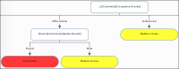
6 Create the remaining classifications. Figure 6‑14 shows three classifications: High income, Medium income, and Low income.
6 Choose Train. A graphical representation of the decision tree appears in Chart. The classifications appear with the names and colors you specified.
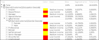
Figure 6‑14 shows part of a decision tree for the Customer table domain with domain columns Occupation Decode and Gender Decode. The decision tree predicts whether a worker is low income, medium income, or high income, based on the worker’s occupation and gender. For professionals, the income classification does not depend on gender. For office workers, however, the classification for men is medium income, while the classification for women is low income.
Figure 6‑14 Graphical representation of a decision tree
7 Choose Browser. A tabular representation of the decision tree appears.
8 Expand the tree. Figure 6‑15 shows a tabular representation of the decision tree, shown graphically in Figure 6‑14.
Figure 6‑15 Tabular representation of a decision tree
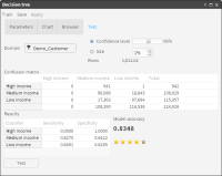
9 Choose Test.
10 Drag the appropriate table from My Data and drop it in Domain.
11 Choose Test. Figure 6‑16 shows the test results.
Figure 6‑16 Test results, including the confusion matrix