Linear regression attempts to model the relationship between variables by fitting a linear equation to observed data. One or more variables are considered to be independent predictors or explanatory variables while the other variable is considered to be a dependent variable.
Linear regression is mainly used for:
Forecasting a dependent variable
Quantifying the level of relationship between a dependent variable and independent predictor variables
Before attempting to fit a linear model to observed data, you first need to determine whether or not there is a relationship or significant association between the chosen variables.
Displaying the data on a scatter plot helps to determine the strength of relationship between two variables. If the scatter plot does not show any increasing or decreasing trends then you should not bother trying to fit a linear regression model to the data.
Least-Squares Regression
The BIRT Analytics Linear Regression tool uses the most effective and well-known method for fitting a regression line. It is called the OLS (Ordinary Least-Squares) algorithm. It calculates the best-fitting line for the observed data by minimizing the sum of the squares of the vertical deviations from each data point to the line (if a point lies exactly on the fitted line its vertical deviation is zero). Because the deviations are first squared then summed, there are no cancellations between positive and negative values. This minimizes error in the dependent variable.
How to make a linear regression
The following procedure show you how to create a linear regression using the BIRT Analytics tool:
1 Click on the Analytics button on the home screen.
2 Open the Advanced tab and choose Linear regression.
3 Expand the database and tables in the Data Tree pane on the left.
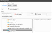
4 Drag the table that you want to analyze from the Data Tree on the left and drop it into the Filter field. This table represents the Domain of the variables to be studied. In this case drag and drop the Customer table into the Filter field.
5 Again from the Data Tree, drag the column that will be used as the dependent variable (on which predictions will be made) and drop it into the Dependent variable field. In this case drag and drop the Total Orders variable. This action automatically populates the Table field on the right.
6 Expand the tables that appear in the left pane of the workspace. Then drag from this pane the columns that you want to use as independent predictor variables and drop them into the empty pane on the right. In this case drag and drop the Total products variable. You can compare your results to Figure 6‑23.
Figure 6‑23 Creating a linear regression
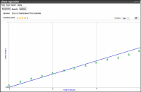
7 Choose Train to make the calculation. This opens the Results tab that gives you the equation that you can apply to any of the Predictor values to predict the dependent variable. There is a graphic display of the function (including the plotted values) which makes it easy to see at a glance that, in this case, it is a very close fit.A set of one or more (or none) gold stars indicate the goodness of fit of your equation, as shown in Figure 6‑24.
Figure 6‑24 Linear regression - Results tab
Understanding advanced statistical values in the Statistics tab
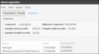
To view more advanced statistical results you can open the Statistics tab for your model, as shown in Figure 6‑25.
Figure 6‑25 Linear regression - Statistics tab
These results are the coefficients that accompany each independent predictor and the intercept. The Interceptor is the value of the dependent variable when all the predictor values are zero.
Each coefficient has additional associated parameters such as:
Standard error
t-stats - associated with the Student-T distribution test - higher values imply that the coefficient is not zero.
P-value - this value shows the results of the hypothesis test as a significance level. Values of less than 0.5 imply that the coefficient is not zero
Upper and lower confidence levels - Assuming that the error in the prediction of the dependent variable is normally distributed, BIRT Analytics is able to calculate the confidence interval of the linear regression. The results are two linear functions with coefficients and intercepts for both the 95% upper confidence level and the 95% lower confidence level, also known as the 95% confidence bands.
For the global results of the linear regression, the statistics that measure the goodness of fit are:
R2 - (R-Squared) - Also known as a coefficient or determination, it indicates how well data provided fits with the linear regression model that has been calculated. Values close to zero indicate no linear relationship.
Adjusted R-Squared- Sometimes R-Squared suffers an increase in its value due to the addition of extra predictors without improving the fit. Adjusted R-Squared will always be less or equal to R2
The Linear regression tool also shows the total records used from the Domain. Invalid records come from those having null values.