In the previous section we described the linear regression model used for predicting relationships between data variables. Although logistic regression also measures relationships based on observed data, it is a much more complex model than linear regression. Logistic regression tries to produce a realistic binary result concerning the likelihood of something occurring (ie. the odds of success) - predicting probability from observed data variables.
Our model predicts a binary response from a binary predictor (explanatory/independent variable) predicts the outcome of a dependent variable based on one or more predictor variables. In other words, it estimates the parameters of a qualitative response model.
In our model the dependent variable is binary which means the available categories is two. It measures the relationship between a categorical dependent variable and one or more independent variables, which are usually continuous. Logistic regression uses probability scores as the predicted values of the dependent variable.
Logistic regression is used in many fields. In the medical field it is often used to predict whether a patient has a particular disease, such as diabetes or coronary heart disease, based on observed patient characteristics such as: age, gender, body mass index, relative weight, blood cholesterol levels, etc.
In marketing it is used to predict customer propensity to purchase a particular product or to cease a subscription, etc. In economics it predicts the rise or fall of unemployment over a coming period. In business and banking it was recently used to predict the likelihood of homeowners defaulting on their sub-prime mortgages (with results that encouraged disastrous behavior in this case). Logistic regression results only predict the odds of success but they cannot guarantee it.
Basic principles
In binary logistic regression the outcome is coded as “0” or “1” which leads to the most straightforward interpretation. If a particular observed outcome for the dependent variable is a relevant possible outcome (often called a “success” or a “case”), it is coded as “1”. The contrary outcome (called a “failure” or “noncase”) is coded as “0”.
Logistic regression predicts the odds of “success” (or the “case”) based on the values of the independent variables (predictors). Mathematically speaking, these odds are defined as the probability that an outcome is a success (or case) divided by the probability that the outcome is a failure (or noncase)
Logistic regression takes the natural logarithm (or “logit”) of the odds of the dependent variable being a successto create a continuous criterion as a transformed version of the dependent variable. This “logit” transformation is called the “link” function in logistic regression. Although the dependent variable in logistic regression is binomial, the “logit” is the continuous criterion where linear regression is conducted.
Once transformed, the ‘logit’ of success is then fit to the predictors using linear regression analysis. The predicted value of the logit is converted back into predicted odds via the inverse of the natural logarithm, the exponential function.
The observed dependent variable in logistic regression is a zero-or-one variable. The logistic regression estimates the odds, as a continuous variable, that the dependent variable is a success.
A categorical prediction can be based on the computed odds of a success, with predicted odds above some chosen cut-off value being translated into a prediction of success.
How to make a logistic regression
The following procedure show you how to create a logistic regression using the BIRT Analytics tool. [In this case we will determine the probability of a customer being female, using as a predictor the total number of purchases made by the customer.]
1 Click on the Analytics button on the home screen.
2 Open the Advanced tab and choose Logistic regression.
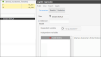
3 Prepare the segment you want to analyze in the Scratchpad by dragging in the desired discrete values from your chosen column in the Data Tree. In this case use the discrete values from the gender column for your segment.
4 Drag the newly created segment “GENDER IM F,M” into the Filter field from the Data Tree. Now two panels appear in the workspace under “Independent variables”, as shown in Figure 6‑26.
Figure 6‑26 Logistic regression - preparing a segment for the Filter field
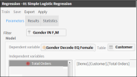
5 Again from the Data Tree, drag the column Gender decode EQ Female and drop it into the Dependent variable field. (Predictions will be made on this variable). This action automatically enters the “Customer” table in the Table field on the right. This table represents the Domain of the variables to be studied, as shown in Figure 6‑27.
Figure 6‑27 Logistic regression - Setting the dependent and predictor variables
6 Expand the tables that appear in the left pane of the workspace. Then drag from this pane the Total Orders column that will be used as an independent predictor variable and drop it into the empty pane on the right, shown in Figure 6‑27.
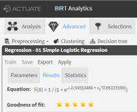
7 Choose Train to make the calculation. This opens the Results tab that gives you the equation that you can apply to any of the Predictor values to predict the dependent variable. The results of the calculation are the coefficients that accompany each predictor and the intercept.
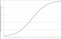
A set of five gold stars indicates that the goodness of fit of your equation is very high. There is also a chart of the function, as shown in Figure 6‑28 and Figure 6‑29.
Figure 6‑28 Logistic regression - results tab
Figure 6‑29 Logistic regression - graphic display of the function
Understanding advanced statistical values in the Statistics tab
For more advanced results, the Statistics tab supports analyzing each calculated coefficient of the equation, their goodness of fit and relevance of the model. You can save the model and apply it to predict values of the dependent variable using the calculated equation.
Each coefficient has additional associated parameters such as:
Standard error
Odds ratio. This ratio quantifies how strongly the presence or absence of certain property is associated with the presence or absence of another property in a given domain. As bigger is the ratio, better is the relationship between dependent variable and the independent related to the coefficient.
Odds Upper and Lower Confidence Level (95%). It has the same calculation as confidence level for a domain mean, but it’s calculated on the natural log scale. It gives two functions to define the confidence interval or band.
Log likelihood p value. The p-value shows the results of the hypothesis test as a significance level. In that case smaller values than 0.5 are taken as evidence that the coefficient is nonzero.
Significance Level. Based on a distinct range of significance values for p-value, it is possible to classify the level of significance of this coefficient.It is a range from 0 to 5, where 0 means no significance and 5 means a highly relevant significance level.
For the global results of logistic regression, the statistics that measure goodness of fit are:
Chi Squared test. Also known as the likelihood ratio test, it’s an asymptotically distributed Chi Squared test with certain degrees of freedom. As bigger is its value, better is the goodness of fit of the model.
Chi Squared p-value. Is the statistical significance testing from the Chi Squared test. The p-value is the probability of obtaining the observed sample results (or a more extreme result) when the null hypothesis is actually true. This shows that when p-value is very small (less than a certain threshold), it tells that the modeled data is inconsistent with the assumption that the null hypotheses is true. In other words, this hypothesis can be rejected, so the modeled data can be accepted as true.
Log likelihood. It’s the logarithm of the likelihood ratio. This will always be negative, with higher values (closer to zero) indicating a better fitting model.
The tool also shows the total records used from the total selected in the Domain. Invalid records come from those that have null values in some variables.