Naive Bayes classification is a type of simple probability classification based on the Bayes algorithm, with a strong hypothesis of independence (called naïve”). It implements a naïve Bayesian classifier, belonging to the family of linear classifiers.
In probability theory and statistics, the Bayes algorithm relates current probability to prior probability. It is important in the mathematical manipulation of conditional probabilities. Bayes’ rule can be derived from more basic axioms of probability, specifically conditional probability.
This algorithm was first used as a method for text categorization, to identify documents as belonging to one category or another (such as spam or legitimate, sports or politics) with word frequencies as the features. It is still competitive in this domain. It also finds useful application in automatic medical diagnosis.
Naïve Bayes classifiers are highly scalable, requiring several parameters that are linear in the number of variables (features/predictors) in a learning problem.Maximum-likelihood training can be done by evaluating aclosed-form expression, which takesnear time, rather than by time consumingiterative approximationas used for many other types of classifiers.
Basic principles
The underlying probability model of the Naïve Bayes classification algorithm is best described as a model with statistically independent characteristics. A naïve Bayesian classifier supposes that the existence of a characteristic for a given class is independent from the existence of the other characteristics for that class.
For example, a fruit can be considered as an apple if it is red and round. Even if these characteristics can often be connected in reality, a naïve Bayesian classifier will determine that the fruit is an apple by considering independently these characteristics of (A) color and (B) shape.
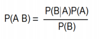
Bayes' theorem is stated mathematically as the following equation:
whereAandBare events.
P(A) and P(B) are theprobabilities ofAandBindependent of each other.
P(A|B), aconditional probability, is the probability ofAgiven thatBis true.
P(B|A), is the probability ofBgiven thatAis true.
In many practical applications, the estimation of the parameters for the naïve Bayesian models is based on maximum likelihood. In spite of their "naïve" design model and its extremely simplistic basic hypotheses, the naïve Bayesian classifiers demonstrated an acceptable level of efficiency in many complex real-world situations.
Advantages
The main advantage of the naïve Bayesian classifier is that it requires relatively little training data. The necessary parameters for the classification are the averages and the variances of the variables. Indeed, the hypothesis of independence of variables does not require knowing more than the variance of each variable for every class, without having to calculate a covariance matrix.
The naive Bayes classifier has several properties that make it surprisingly useful. In particular, the decoupling of the class conditional feature distributions means that each distribution can be independently estimated as a one-dimensional distribution. This helps alleviate problems stemming from thedifficulties of dimensionality, such as the need for data sets that scale exponentially with the number of features.
Relation to Linear and Logistic Regression
In statistics, Bayesian linear regression is an approach to linear regression in which the statistical analysis is undertaken in the context of Bayesian inference. When the regression model has errors that have a normal distribution, and if a particular form of prior distribution is assumed, explicit results are available for the posterior probability distributions of the model’s parameters.
In the case of discrete inputs (indicator or frequency features for discrete events), naïve Bayes classifiers form a generative-discriminative pair with (multinomial) logistic regression classifiers: each naïve Bayes classifier can be considered to be a way of fitting a probability model that optimizes the joint likelihood p(C,x), while logistic regression fits the same probability model to optimize the conditionalp(CIx).
The link between the two can be seen by observing that the decision function for naïve Bayes (in the binary case) can be rewritten as “predict class C1if the odds of p(C1Ix) exceed those of p(C2Ix).
Expressing this in log-space gives:
The left-hand side of this equation is the log-odds, or logit, the quantity predicted by the linear model that underlies logistic regression. Since naïve Bayes is also a linear model for the two “discrete” event models, its parameters can be re-set as a linear function:
Obtaining the probabilities is then a matter of applying the logistic function to b + wTx, or in the multiclass case, the softmax function.
Although discriminative classifiers have lower asymptotic error than generative ones, in many practical cases naive Bayes can outperform logistic regression because it reaches its asymptotic error faster.
How to make a Naive Bayes classification
1 Click on the Analytics button on the home screen.
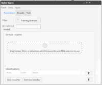
2 Open the Advanced tab and choose NaIve Bayes. This opens the screen where you set your parameters. (See Figure 6‑30).
Figure 6‑30 Configuration screen in the Parameters tab
3 In the “Parameters” tab, set the Training domain by dragging the appropriate table from the Data Tree and dropping it into the “Filters” field. Here we chose: [Demo].[Customer].[Customer Profit Decile] EQ 1 OR 10.
4 In the left-hand panel of the “Domain columns” field, expand the Database tree and its appropriate tables. Then drag the desired Domain columns from this expanded tree into the right-hand panel of the field.These columns specify the attributes used to assign classifications in Naive Bayes. Here we chose: Age Numeric, Gender Decode, Income Numeric and Occupation Decode.
5 We are now ready to create our first classifier by clicking on the “New classifier” button. This opens the configuration fields in the lower right-hand side of the screen. Now drag the segment “Customer Profit Decile EQ10” into the “drag a segment” field.
6 Type the name of your classifier in the “Alias” field and choose your color via the color palette icon. Here we named our classifier “High Profit” and choose a rusty brown for its color via the icon beside the color block, as shown in Figure 6‑31. Now choose “OK”.
Figure 6‑31 “New classifier” configuration fields
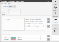
7 Repeat the operation to set the second classifier “Customer Profit Decile EQ1” naming it “Low Profit”, select a teal green color and choose “OK” again. Now you are back in the main configuration screen that now displays your parameters, as shown in Figure 6‑32.
Figure 6‑32 Configured parameters for Naive Bayes analysis
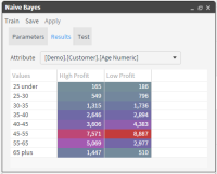
8 Click “Train” in the toolbar to see your results, as shown in Figure 6‑33.
Figure 6‑33 Naive Bayes analysis results
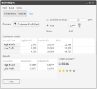
9 Now test the accuracy of your results in the “Test” tab by dragging your classifier segments into the “Domain” field and clicking “Test” at the bottom of the screen, as shown in Figure 6‑34.
Note: To obtain the most useful results, it would be wise to find the best classifier by comparing the same Domain, Classifiers and Domain Columns in both a Decision Tree and a Naive Bayes analysis.
Figure 6‑34 Test results including the confusion matrix
Useful Guidelines when building Naive Bayes classifications
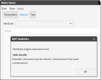
When training in Naive Bayes, the classifier domains must be disjoint, otherwise an error message is displayed. (See Figure 6‑35). This means that each register in the Filter domain has to be linked with only one classifier.
Figure 6‑35 Alert received if chosen classifiers intersect
Although no official size limitation exists concerning the discrete values that a Domain column can contain, the User can sometimes receive the following Alert when using a particular high volume Domain column in an analysis: “Not enough memory.”
The alert also indicates the bytes requested compared to the bytes available (for example: 10000000 bytes requested, but only 3797856 are available).
If this message appears, it is necessary to use a Domain column with fewer discrete values, such as replacing an “Income” column with an “Income numeric” or an “Age” column with an “Age numeric” column, etc.