Using evolution
An evolution analysis shows a progression of data over time. You can examine the behavior of certain measures in different periodic scenarios. For example, examine how the sales of some product families evolve over a period of months. The product family field is the categorical variable under study, while the different scenarios are determined by the different values in the month of purchase variable.
Define the following components to create an evolution analysis:

Categorical variable: Field that contains the categories whose behavior is to be analyzed, or in other words, the variable under study.
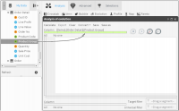
To indicate the variable you want to work with, drag the field from Data Tree to the control that is in the top part of the configuration form, as shown in
Figure 4‑18.
Figure 4‑18 Control without variables
After dragging the variable to the control, it checks the number of discrete values and shows all of the divisions as well as the single values that it contains, as shown in
Figure 4‑19. Each green strip corresponds to a product type.
Figure 4‑19 Control with variables
You can drag to this control only fields with a maximum of 100 discrete values. In the analysis, a sphere with a specific color selected at random represents each of these categories.
If you want to delete one or more of the categories from the analysis variable, click the box that represents the category. If you position the cursor over each of the green boxes, a tag appears, displaying the value of the option.
You can also select or deselect all of the boxes by using the buttons located just below the discrete values control (all, none).
Measures: Evolution can display up to a maximum of three measures, two of which position the spheres on the axes of the
x‑ and
y‑ coordinates, while the third (optional) defines the relative measure of the sphere inside the group.
To define the measures of the axes, drag the numeric fields from Data Tree to the vertical bar (y-axis) or to the horizontal bar (x-axis).
When you drag a column to the x-axis, the latter changes color, indicating that it is ready to accept a column. After you drop the field, the control shows the applicable functions available in accordance with the type of column.
To use the third measure (sphere measure), drag the column you want to use to the icon that is located in the top‑right part of the form.
If the cursor is positioned over the definition controls of the measures (axes, measure control), the current operation as well as the field involved in it are displayed.
Transition variable: It is necessary to define what data tree variable to use as a base for creating transitions. To indicate the field, you drag it to the discrete values control at the bottom of the form.
This control operates in the same way as the categorical variable control and enables you to indicate which elements to use in the analysis.
How to create an evolution
1 In Analytics—Analysis, choose Evolution.
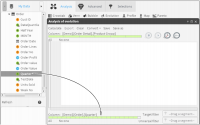
2 From Data Tree, drag a column to use as the categorical variable, as shown in
Figure 4‑20.
Figure 4‑20 Defining a categorical variable for an evolution analysis
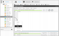
3 From Data Tree, drag a column to use as the transition variable, as shown in
Figure 4‑21.
Figure 4‑21 Defining a transition variable for an evolution analysis
4 From Data Tree, drag columns onto the
x-axis and
y-axis. Choose appropriate functions for each axis.
Figure 4‑22 shows the
y-axis being added as mean order profit with the x‑axis in blue, to indicate that a column has already been applied.
Figure 4‑22 Defining y-axis properties for an evolution analysis
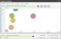
5 Choose Calculate. Choose Play to show the evolution over time.
Figure 4‑23 shows the evolution analysis.
Figure 4‑23 Viewing an evolution analysis
6 To indicate a third measure, from Data Tree, drag a column to the far right icon.
7 To modify the transition of time, select the clock icon and choose an interval. For example, an interval of 0.25 is faster than an interval of 3.