Understanding sensitivity and specificity
Sensitivity, also called the true positive rate, measures the proportion of actual positives that are correctly identified as such, for example the percentage of sick people who are correctly identified as having a condition. Specificity, also called the true negative rate, measures the proportion of negatives that are correctly identified as such, for example the percentage of healthy people who are correctly identified as not having a condition. A perfect predictor is 100% sensitive, in other words predicting that all people in the sick group are sick, and 100% specific, in other words not predicting that anyone in the healthy group is sick. For any test, however, there is a trade-off between the measures. For example, in an airport security setting where one is testing for potential threats to safety, scanners may be set to trigger on low-risk items such as belt buckles and keys, low specificity, in order to reduce the risk of missing objects that pose a threat to passengers and crew, high sensitivity.
How to create a decision tree
1 In Analytics—Advanced, choose Decision tree.
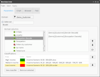
2 Drag the appropriate table from My Data and drop it in Domain in Decision tree, shown in
Figure 6‑13.
3 In the left pane of Domain columns, expand the database and the appropriate tables.
4 Drag the appropriate columns from the left pane and drop them in the right pane. The columns specify the attributes used to assign classifications in the decision tree.
5 Create the classifications:
1 Choose New classifier.
2 In Alias, type the name of the classifier.
3 Choose the color picker button and select a color. The name and the color visually identify the classification in the decision tree. For example, you can define a High income classification identified by the color green.
4 Drag a segment from Discrete values and drop it in Drag a segment. The segment specifies the condition for the classification. For example, you can define a High income classification as income over 80000.
5 Choose the check mark. The classification appears in Classifications.
6 Create the remaining classifications.
Figure 6‑13 shows three classifications: High income, Medium income, and Low income.
Figure 6‑13 Specifying the parameters for a decision tree
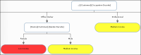
6 Choose Train. A graphical representation of the decision tree appears in Chart. The classifications appear with the names and colors you specified.
Figure 6‑14 shows part of a decision tree for the Customer table domain with domain columns Occupation Decode and Gender Decode. The decision tree predicts whether a worker is low income, medium income, or high income, based on the worker’s occupation and gender. For professionals, the income classification does not depend on gender. For office workers, however, the classification for men is medium income, while the classification for women is low income.
Figure 6‑14 Graphical representation of a decision tree
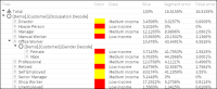
7 Choose Browser. A tabular representation of the decision tree appears.
8 Expand the tree.
Figure 6‑15 shows a tabular representation of the decision tree, shown graphically in
Figure 6‑14.
Figure 6‑15 Tabular representation of a decision tree
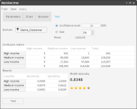
9 Choose Test.
10 Drag the appropriate table from My Data and drop it in Domain.
Figure 6‑16 Test results, including the confusion matrix
Video tutorials