How to set conditional formats
1 To define the condition, right-click a cross tab element on which to display conditional formatting. From the menu, choose Format➛Conditional Formatting.
2 In Conditional Formatting, as shown in
Figure 2‑20, create a rule specifying the following information:

The condition that must be true to apply the format, such as revenue greater than or equal to 45000, as shown in
Figure 2‑20.
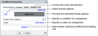
Figure 2‑20 Defining conditional formatting
Choose Font to select formatting attributes.
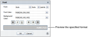
In Font, set formatting attributes:
Select font, size, color, and background color.
Select styles: bold, italic, or underline.
Select an alignment option: Align Left, Align Center, or Align Right.
Figure 2‑21 displays the choices of white text color (RGB(255,255,255)), gray background color (RGB(192,192,192)), and bold style on Font.
Figure 2‑21 Setting font formatting options
Choose OK.
3 In Conditional Formatting, choose OK. In the cross tab in
Figure 2‑22, revenue values greater than or equal to $45,000 appear as bold, white text on a gray background.
Figure 2‑22 Highlighting revenue values greater than or equal to $45,000
4 To add another rule, right-click a cell and choose Format➛Conditional Formatting. Then, on Conditional Formatting, choose Add Rule.
Conditional Formatting displays fields for you to provide a new rule.
How to delete a conditional formatting rule
1 Right-click a cross tab element. From the menu, choose Format➛Conditional Formatting.
2 In Conditional Formatting, choose Delete Rule for each conditional formatting rule that you want to remove. Choose OK.